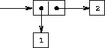
pair(1,
     pair(2,
          pair(3,
               pair(4,[]))))
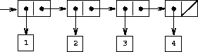
var one_through_four = list(1,2,3,4);
head(one_through_four)
tail(one_through_four)
head(tail(one_through_four))
pair(10,one_through_four)
pair(5,one_through_four)
 and returns the
  th item of the list. It is customary to
number the elements of the list beginning with 0. The method for
computing list_ref is the following:
th item of the list. It is customary to
number the elements of the list beginning with 0. The method for
computing list_ref is the following:
 , list_ref should return the head of the list.
 st item of the
tail of the list.
st item of the
tail of the list.
function list_ref(items,n) {
   if (n === 0)
      return head(items);
   else return list_ref(tail(items),n - 1);
}
function length(items) {
   if (is_empty_list(items))
      return 0;
   else return 1 + length(tail(items));
}
function length(items) {
   function length_iter(a,count) {
      if (is_empty_list(a))
         return count;
      else return length_iter(tail(a),count + 1);
   }
   return length_iter(items,0);
}
append(squares,odds)
append(odds,squares)
function append(list1,list2) {
   if (is_empty_list(list1))
      return list2;
   else return pair(head(list1),append(tail(list1),list2));
}
// last_pair to be given by student
last_pair(list(23,72,149,34))
reverse(list(1,4,9,16,25))
Consider the change-counting program of section 1.2.2. It would be nice to be able to easily change the currency used by the program, so that we could compute the number of ways to change a British pound, for example. As the program is written, the knowledge of the currency is distributed partly into the function first_denomination and partly into the function count_change (which knows that there are five kinds of U.S. coins). It would be nicer to be able to supply a list of coins to be used for making change.
We want to rewrite the function cc so that its second argument is a list of the values of the coins to use rather than an integer specifying which coins to use. We could then have lists that defined each kind of currency:
var us_coins = list(50,25,10,5,1);
var uk_coins = list(100,50,20,10,5,2,1,0.5);
We could then call cc as follows:
cc(100,us_coins)To do this will require changing the program cc somewhat. It will still have the same form, but it will access its second argument differently, as follows: ;; first define first-denomination, except-first-denomination, and no-more // first define first_denomination, except_first_denomination, and no_more
function cc(amount,coin_values) {
   if (amount === 0) return 1;
   else if (amount < 0 || no_more(coin_values)) return 0;
   else return cc(amount,except_first_denomination(coin_values))
               +
               cc(amount - first_denomination(coin_values),
                  coin_values);
}
Define the functions first_denomination, except_first_denomination, and no_more in terms of primitive operations on list structures. Does the order of the list coin_values affect the answer produced by cc? Why or why not?
The function list takes an arbitrary number of arguments. In order to define such a function, we make use of two features of JavaScript. Firstly, note that the JavaScript interpreter tolerates additional arguments to be passed to any function. Thus,
function f(x,y) {
   return x + y;
}
f(1,2,3,4);
will return the number 3.
Secondly, the variable arguments can be used in any function body to refer to all actual arguments. The actual arguments are represented by arguments as an array, and thus available using the notation arguments[0], arguments[1], etc. For example,
function g() {
   return arguments[0] + arguments[1] + arguments[2];
}
f(1,2,3,4);
will return the number 6.
Use this notation to write a function same_parity that takes one or more integers and returns a list of all the arguments that have the same even-odd parity as the first argument. For example,
same_parity(1,2,3,4,5,6,7)returns [1,3,5,7], and
same_parity(2,3,4,5,6,7)returns [2,4,6].
function scale_list(items,factor) {
   if (is_empty_list(items)) return [];
   else return pair(head(items) * factor,
                    scale_list(tail(items),factor));
}
scale_list(list(1,2,3,4,5),10)
function map(fun,items) {
   if (is_empty_list(items))
      return [];
   else return pair(fun(head(items)),
                    map(fun,tail(items)));
}
map(abs,list(-10,2.5,-11.6,17))
map(function(x) { return x * x; },
    list(1,2,3,4))
function scale_list(items,factor) {
   return map(function(x) { return x * factor; },
              items);
}
// square_list to be given by student
square_list(list(1,2,3,4))
Here are two different definitions of square_list. Complete both of them by filling in the missing expressions:
function square_list(items) {
   function iter(things,answer) {
      if (is_empty_list(things))
         return answer;
      else return iter(tail(things),
                       pair(square(head(things)),
                            answer));
   }
   return iter(items,[]);
}
Unfortunately, defining square_list this way produces the answer
list in the reverse order of the one desired. Why?
Louis then tries to fix his bug by interchanging the arguments to
pair:
function square_list(items) {
   function iter(things,answer) {
      if (is_empty_list(things))
         return answer;
      else return iter(tail(things),
                       pair(answer,
                            square(head(things))));
   }
   return iter(items,[]);
}
This doesn’t work either. Explain.
for_each(function(x) { newline(); display(x); },
         list(57,321,88));
The value returned by the call to for_each (not illustrated above)
can be something arbitrary, such as true. Give an
implementation of for_each.
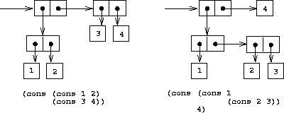
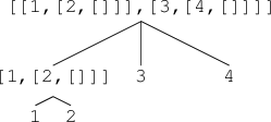
pair(list(1,2),list(3,4))as a list of three items, the first of which is itself a list, [1,[2,[]]]. Figure 2.5 shows the representation of this structure in terms of pairs.
|
|
var x = [[1,[2,[]]],[3,[4,[]]]];
length(x)
count_leaves(x)
list(x,x)
length(list(x,x))
count_leaves(list(x,x))
function count_leaves(x) {
   if (is_empty_list(x))
      return 0;
   else if (! is_pair(x))
      return 1;
   else return count_leaves(head(x)) +
               count_leaves(tail(x));
}
var x = list(1,2,3);

var y = list(1,2,3);
What result is printed by the interpreter in response to evaluating each of the following expressions:
append(x,y)
pair(x,y)
list(x,y)
var x = list(list(1,2),list(3,4));Here,
xshould return
reverse(x)should return whereas
deep_reverse(x)should return
var x = list(list(1,2),list(3,4))Here,
fringe(x)should return and
fringe(list(x,x))should return
function make_mobile(left,right) {
   return list(left,right);
}
A branch is constructed from a length (which must be a number)
together with a structure, which may be either a number
(representing a simple weight) or another mobile:
function make_branch(length,structure) {
   return list(length,structure);
}
function make_mobile(left,right) {
   return pair(left,right);
}
function make_branch(length,structure) {
   return pair(length,structure);
}
How much do you need to change your programs to convert to the new
representation?
function scale_tree(tree,factor) {
   if (is_empty_list(tree))
      return [];
   else if (! is_pair(tree))
      return tree * factor;
   else return pair(scale_tree(head(tree),factor),
                    scale_tree(tail(tree),factor));
}
scale_tree(list(1,list(2,list(3,4),5),list(6,7)),
           10)
function scale_tree(tree,factor) {
   return map(function(sub_tree) {
                 if (is_pair(sub_tree))
                    return scale_tree(sub_tree,factor);
                 else
                    return sub_tree * factor;
              },
              tree);
}
square_tree(list(1,
                 list(2,list(3,4),5),
                 list(6,7)))
should return
Define square_tree both directly (i.e., without using any
higher-order
functions) and also by using map and recursion.
function square_tree(tree) {
   return tree_map(square,tree);
}
function subsets(s) {
   if (is_empty_list(s))
      return list([]);
   else {
      var rest = subsets(tail(s));
      return append(rest,map(^??^,rest));
   }
}
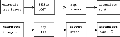
function sum_odd_squares(tree) {
   if (is_empty_list(tree))
      return 0;
   else if (! is_pair(tree))
      return (is_odd(tree)) ? square(tree) : 0;
   else return sum_odd_squares(head(tree))
               +
               sum_odd_squares(tail(tree));
}
 , where
  is less than or equal to a given integer
  :
:
function even_fibs(n) {
   function next(k) {
      if (k > n)
         return [];
      else {
         var f = fib(k);
         if (is_even(f))
            return pair(f,next(k+1));
         else return next(k+1);
      }
   }
   return next(0);
}
 ;
;
map(square,list(1,2,3,4,5))
function filter(predicate,sequence) {
   if (is_empty_list(sequence))
      return [];
   else if (predicate(head(sequence)))
      return pair(head(sequence),
                  filter(predicate,tail(sequence)));
   else
      return filter(predicate,tail(sequence));
}
filter(is_odd,list(1,2,3,4,5))Accumulations can be implemented by
function accumulate(op,initial,sequence) {
   if (is_empty_list(sequence))
      return initial;
   else
      return op(head(sequence),
                accumulate(op,initial,tail(sequence)));
}
accumulate(plus,0,list(1,2,3,4,5))
accumulate(times,1,list(1,2,3,4,5))
accumulate(pair,[],list(1,2,3,4,5))
function enumerate_interval(low,high) {
   if (low > high)
      return [];
   else
      return pair(low,
                  enumerate_interval(low+1,high));
}
enumerate_interval(2,7)
function enumerate_tree(tree) {
   if (is_empty_list(tree))
      return [];
   else if (! is_pair(tree))
      return list(tree);
   else
      return append(enumerate_tree(head(tree)),
                    enumerate_tree(tail(tree)));
}
enumerate_tree(list(1,list(2,list(3,4)),5))
function sum_odd_squares(tree) {
   return accumulate(plus,
                     0,
                     map(square,
                         filter(is_odd,
                                enumerate_tree(tree))));
}
 , generate
the Fibonacci number for each of these integers, filter the resulting
sequence to keep only the even elements, and accumulate the results
into a list:
, generate
the Fibonacci number for each of these integers, filter the resulting
sequence to keep only the even elements, and accumulate the results
into a list:
function even_fibs(n) {
   return accumulate(pair,
                     [],
                     filter(is_even,
                            map(fib,
                                enumerate_interval(0,n))));
}
 Fibonacci numbers:
function list_fib_squares(n) {
   return accumulate(pair,
                     [],
                     map(square,
                         map(fib,
                             enumerate_interval(0,n))));
}
list_fib_squares(10)
function product_of_squares_of_odd_elements(sequence) {
   return accumulate(times,
                     1,
                     map(square,
                         filter(is_odd,sequence)));
}
product_of_squares_of_odd_elements(list(1,2,3,4,5))
function map(p,sequence) {
   return accumulate(function(x,y) { ?? },
                     [], sequence);
}

function append(seq1,seq2) {
   return accumulate(pair, ??, ??);
}

function length(sequence) {
   return accumulate(??, 0, sequence);
}
 at a given value of
  can be
formulated as an accumulation. We evaluate the polynomial
can be
formulated as an accumulation. We evaluate the polynomial


 , multiply by
  , add
, add  ,
multiply by
,
multiply by  , and so on, until we reach
  .11
Fill in the following template to produce a
function
that evaluates a
polynomial using Horner’s rule.
Assume that the coefficients of the
polynomial are arranged in a sequence, from
.11
Fill in the following template to produce a
function
that evaluates a
polynomial using Horner’s rule.
Assume that the coefficients of the
polynomial are arranged in a sequence, from  through
  .
.
function horner_eval(x,coefficient_sequence) {
   return accumulate(function(this_coeff,
                              higher_terms) {
                        ??
                     },
                     0,
                     coefficient_sequence);
}
For example, to compute 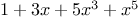 at
at  you would evaluate
horner_eval(2,list(1,3,0,5,0,1))
function count_leaves(t) {
   return accumulate(??, ??, map(??, ??));
}
function accumulate_n(op,init,seqs) {
   if (is_empty_list(head(seqs)))
      return [];
   else
      return pair(accumulate(op,init,??),
                  accumulate_n(op,init,??));
}
 as sequences of numbers, and
matrices
as sequences of numbers, and
matrices  as sequences of vectors (the rows of the matrix).
For example, the matrix
as sequences of vectors (the rows of the matrix).
For example, the matrix
 ,
, ) returns the sum
  .
.
 ,
, ) returns the vector
  , where
  .
.
 ,
, ) returns the matrix
  , where
  .
.
 ) returns the matrix
  , where
  .
.
function dot_product(v,w) {
   return accumulate(plus,0,map(times,v,w));
}
Fill in the missing expressions in the following
functions
for
computing the other matrix operations. (The
function
accumulate_n is
defined in exercise 2.37.)
function matrix_times_vector(m,v) {
   return map(??,m);
}

function transpose(mat) {
   return accumulate_n(??,??,mat);
}

function matrix_times_matrix(n,m) {
   var cols = transpose(n);
   return map(??,m);
}
function fold_left(op,initial,sequence) {
   function iter(result,rest) {
      if (is_empty_list(rest))
         return result;
      else
         return iter(op(result,head(rest)),
                     tail(rest));
   }
   return iter(initial,sequence);
}
What are the values of
fold_right(divide,1,list(1,2,3))
fold_left(divide,1,list(1,2,3))
fold_right(list,[],list(1,2,3))
fold_left(list,[],list(1,2,3))Give a property that op should satisfy to guarantee that fold_right and fold_left will produce the same values for any sequence.
function reverse(sequence) {
   return fold_right(function(x,y) { ?? },[],sequence);
}

function reverse(sequence) {
   return fold_left(function(x,y) { ?? },[],sequence);
 , find all ordered pairs of
distinct positive integers
, find all ordered pairs of
distinct positive integers  and
and  , where
  , such
that
, such
that  is prime. For example, if
  is 6, then the pairs are
the following:
is 6, then the pairs are
the following:
 ,
filter to select those pairs whose sum is prime, and
then, for each pair
,
filter to select those pairs whose sum is prime, and
then, for each pair  that passes through the filter, produce the triple
 .
.
 , enumerate the integers
  , and for each such
  and
and  generate the pair
  . In terms of sequence operations, we map
along the sequence enumerate_interval(1,n). For each
. In terms of sequence operations, we map
along the sequence enumerate_interval(1,n). For each  in
this sequence, we map along the sequence enumerate_interval(1,i-1). For each
in
this sequence, we map along the sequence enumerate_interval(1,i-1). For each  in this latter sequence, we generate the pair
list(i,j). This gives us a sequence of pairs for each
in this latter sequence, we generate the pair
list(i,j). This gives us a sequence of pairs for each  .
Combining all the sequences for all the
.
Combining all the sequences for all the  (by accumulating with append) produces the required sequence of pairs:14
accumulate(append,
           [],
           map(function(i) {
                  return
                     map(function(j) {
                            return list(i,j);
                         },
                         enumerate_interval(1,i-1))
               },
               enumerate_interval(1,n)))
function flatmap(proc,seq) {
   return accumulate(append,[],map(proc,seq));
}
function is_prime_sum(pair) {
   return is_prime(head(pair)+head(tail(pair)));
}
function make_pair_sum(pair) {
   return list(head(pair),head(tail(pair)),
               head(pair)+head(tail(pair)));
}
function prime_sum_pairs(n) {
   return map(make_pair_sum,
              filter(is_prime_sum,
                     flatmap(function(i) {
                                return map(function(j) {
                                              return list(i,j);
                                           },
                                           enumerate_interval(1,i-1));
                             },
                             enumerate_interval(1,n))));
}
 ; that is, all the ways of ordering the items in
the set. For instance, the permutations of
; that is, all the ways of ordering the items in
the set. For instance, the permutations of  are
are
 ,
,  ,
,  ,
,  ,
,  , and
, and
 . Here is a plan for generating the permutations of
  :
For each item
:
For each item  in
in  , recursively generate the sequence of
permutations of
, recursively generate the sequence of
permutations of  ,15 and adjoin
 to the front of each one. This yields, for each
  in
in  , the sequence
of permutations of
, the sequence
of permutations of  that begin with
  . Combining these
sequences for all
. Combining these
sequences for all  gives all the permutations of
  :16
:16
function permutations(s) {
   if (is_empty_list(s))
      return list([]);
   else
      return flatmap(function(x) {
                        return map(function(p) {
                                      return pair(x,p);
                                   },
                                   permutations(remove(x,s)));
                     },
                     s);
}
 to the problem of generating the permutations of
sets with fewer elements than
to the problem of generating the permutations of
sets with fewer elements than  . In the terminal case, we work our
way down to the empty list, which represents a set of no elements.
For this, we generate list([]), which is a sequence with one
item, namely the set with no elements. The remove
function
used in permutations returns all the items in a given sequence
except for a given item. This can be expressed as a simple filter:
. In the terminal case, we work our
way down to the empty list, which represents a set of no elements.
For this, we generate list([]), which is a sequence with one
item, namely the set with no elements. The remove
function
used in permutations returns all the items in a given sequence
except for a given item. This can be expressed as a simple filter:
function remove(item,sequence) {
   return filter(function(x) {
                    return ! (x === item);
                 },
                 sequence);
}
 ,
generates the sequence of pairs
,
generates the sequence of pairs  with
with  . Use unique_pairs to simplify the definition of prime_sum_pairs
given above.
. Use unique_pairs to simplify the definition of prime_sum_pairs
given above.
 ,
,  , and
, and  less than or
equal to a given integer
less than or
equal to a given integer  that sum to a given integer
  .
.
 queens, we must place the
  th queen in a
position where it does not check any of the queens already on the
board. We can formulate this approach recursively: Assume that we
have already generated the sequence of all possible ways to place
th queen in a
position where it does not check any of the queens already on the
board. We can formulate this approach recursively: Assume that we
have already generated the sequence of all possible ways to place
 queens in the first
  columns of the board. For each of
these ways, generate an extended set of positions by placing a queen
in each row of the
columns of the board. For each of
these ways, generate an extended set of positions by placing a queen
in each row of the  th column. Now filter these, keeping only
the positions for which the queen in the
th column. Now filter these, keeping only
the positions for which the queen in the  th column is safe with
respect to the other queens. This produces the sequence of all ways
to place
th column is safe with
respect to the other queens. This produces the sequence of all ways
to place  queens in the first
  columns. By continuing this
process, we will produce not only one solution, but all solutions to
the puzzle.
We implement this solution as a
function
queens, which returns
a sequence of all solutions to the problem of placing
columns. By continuing this
process, we will produce not only one solution, but all solutions to
the puzzle.
We implement this solution as a
function
queens, which returns
a sequence of all solutions to the problem of placing  queens on an
 chessboard. The function queens has an internal
function
queens_cols that returns the sequence of all ways to place queens in
the first
chessboard. The function queens has an internal
function
queens_cols that returns the sequence of all ways to place queens in
the first  columns of the board.
function queeens(board_size) {
   function queen_cols(k) {
      if (k===0)
         return list(empty_board);
      else
         return filter(function(positions) {
                          return is_safe(k,positions);
                       },
                       flatmap(function(rest_of_queens) {
                                  return map(function(new_row) {
                                                return adjoin_position(new_row,
                                                                       k,
                                                                       rest_of_queens);
                                             },
                                             enumerate_interval(1,board_size));
                               },
                               queens_cols(k-1)));
   }
   return queen_cols(board_size);
}
In this
function
rest_of_queens is a way to place  queens
in the first
queens
in the first  columns, and new_row is a proposed row in
which to place the queen for the
columns, and new_row is a proposed row in
which to place the queen for the  th column. Complete the program
by implementing the representation for sets of board positions,
including the
function
adjoin_position, which adjoins a new row-column
position to a set of positions, and empty_board, which
represents an empty set of positions. You must also write the
function
is_safe, which determines for a set of positions,
whether the queen in the
th column. Complete the program
by implementing the representation for sets of board positions,
including the
function
adjoin_position, which adjoins a new row-column
position to a set of positions, and empty_board, which
represents an empty set of positions. You must also write the
function
is_safe, which determines for a set of positions,
whether the queen in the  th column is safe with respect to the
others. (Note that we need only check whether the new queen is
safe—the other queens are already guaranteed safe with respect to
each other.)
th column is safe with respect to the
others. (Note that we need only check whether the new queen is
safe—the other queens are already guaranteed safe with respect to
each other.)
 case.) When Louis asks Eva Lu Ator for help, she points
out that he has interchanged the order of the nested mappings in the
flatmap, writing it as
Explain why this interchange makes the program run slowly. Estimate
how long it will take Louis’s program to solve the eight-queens
puzzle, assuming that the program in exercise 2.43 solves
the puzzle in time
case.) When Louis asks Eva Lu Ator for help, she points
out that he has interchanged the order of the nested mappings in the
flatmap, writing it as
Explain why this interchange makes the program run slowly. Estimate
how long it will take Louis’s program to solve the eight-queens
puzzle, assuming that the program in exercise 2.43 solves
the puzzle in time  .
.
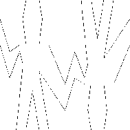
|
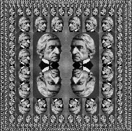
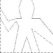
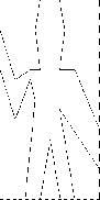
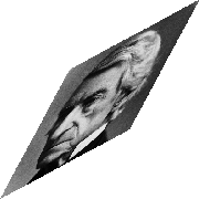
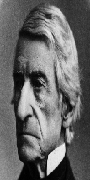
wave(full_frame);Painters can be more elaborate than this: The primitive painter called rogers paints a picture of MIT’s founder, William Barton Rogers, as shown in figure 2.11.18
rogers(full_frame);Our Javascript environment provides a function make_painter_from_url, which generates a painter for the picture that can be obtained using a given URL (Uniform Resource Locator).
var bird = make_painter_from_url(
           "http://www.comp.nus.edu.sg/~henz/sicp/img_original/bird.gif");
bird(full_frame);


|
|
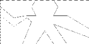
var wave2 = beside(wave,flip_vert(wave));
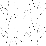
var wave4 = below(wave2,wave2);
var wave4 = flipped_pairs(wave);
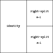
function right_split(painter,n) {
   if (n === 0)
      return painter;
   else {
      var smaller = right_split(painter,n - 1);
      return beside(painter,below(smaller,smaller));
   }
}
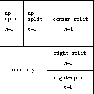
function corner_split(painter,n) {
   if (n === 0)
      return painter;
   else {
      var up = up_split(painter,n-1);
      var right = right_split(painter,n-1);
      var top_left = beside(up,up);
      var bottom_right = below(right,right);
      var corner = corner_split(painter,n-1);
      return beside(below(painter,top_left),
                    below(bottom_right,corner));
   }
}
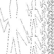
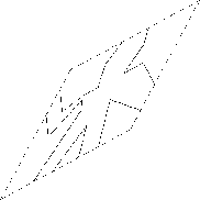
right_split(wave,4) 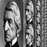
right_split(rogers,4) 
corner_split(wave,4) 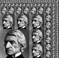
corner_split(rogers,4) |
function square_limit(painter,n) {
   var quarter = corner_split(painter,n);
   var half = beside(flip_horiz(quarter),quarter);
   return below(flip_vert(half),half);
}
function square_of_four(tl,tr,bl,br) {
   return function(painter) {
             var top = beside(tl(painter),tr(painter));
             var bottom = beside(bl(painter),br(painter));
             return below(bottom,top);
          }
}
Then flipped_pairs can be defined in terms
of square_of_four as follows:19
function flipped_pairs(painter) {
   var combine4 = square_of_four(identity,flip_vert,
                                 identity,flip_vert);
   return combine4(painter);
}
and square_limit can be expressed as20
function square_limit(painter,n) {
   var combine4 = square_of_four(flip_horiz,identity,
                                 rotate180,flip_vert);
   return combine4(corner_split(painter,n));
}
 )
to specify images.
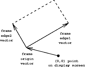
With each frame, we associate a
frame coordinate map, which
will be used to shift and scale images to fit the frame. The map
transforms the unit square into the frame by
mapping the vector
)
to specify images.
With each frame, we associate a
frame coordinate map, which
will be used to shift and scale images to fit the frame. The map
transforms the unit square into the frame by
mapping the vector  to the vector sum

 is mapped to the origin of the frame,
  to
the vertex diagonally opposite the origin, and
to
the vertex diagonally opposite the origin, and  to the
center of the frame. We can create a frame’s coordinate map with the
following
function:21
to the
center of the frame. We can create a frame’s coordinate map with the
following
function:21
function frame_coord_map(frame) {
   return function(v) {
             return add_vect(origin_frame(frame),
                             add_vect(scale_vect(xcor_vect(v),
                                                 edge1_frame(frame)),
                                      scale_vect(ycor_vect(v),
                                                 edge2_frame(frame))));
          };
}
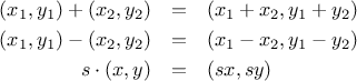
 running from the origin to a point
can be represented as a pair
consisting of an
running from the origin to a point
can be represented as a pair
consisting of an  -coordinate and a
  -coordinate. Implement a data
abstraction for vectors by giving a constructor
make_vect and
corresponding selectors
xcor_vect and
ycor_vect. In
terms of your selectors and constructor, implement
functions
add_vect,
sub_vect, and
scale_vect that perform
the operations vector addition, vector subtraction, and multiplying a
vector by a scalar:
-coordinate. Implement a data
abstraction for vectors by giving a constructor
make_vect and
corresponding selectors
xcor_vect and
ycor_vect. In
terms of your selectors and constructor, implement
functions
add_vect,
sub_vect, and
scale_vect that perform
the operations vector addition, vector subtraction, and multiplying a
vector by a scalar:
function segments_to_painter(segment_list) {
   return function(frame) {
             return for_each(function(segment) {
                                return draw_line(frame_coord_map(frame)(start_segment(segment)),
                                                 frame_coord_map(frame)(end_segment(segment)));
                             },
                             segment_list);
          };
}
function transform_painter(painter,origin,corner1,corner2) {
   return function(frame) {
             var m = frame_coord_map(frame);
             var new_origin = m(origin);
             return painter(make_frame(new_origin,
                                       sub_vect(m(corner1),new_origin),
                                       sub_vect(m(corner2),new_origin)));
          };
}
Here’s how to flip painter images vertically:
function flip_vert(painter) {
   return transform_painter(painter,
                            make_vect(0.0,1.0),  // new origin
                            make_vect(1.0,1.0),  // new end of edge1
                            make_vect(0.0,0.0)); // new end of edge2
}
function shrink_to_upper_right(painter) {
   return transform_painter(painter,
                            make_vect(0.5,0.5),
                            make_vect(1.0,0.5),
                            make_vect(0.5,1.0));
}
Other transformations rotate images counterclockwise by 90 degrees24
function rotate90(painter) {
   return transform_painter(painter,
                            make_vect(1.0,0.0),
                            make_vect(1.0,1.0),
                            make_vect(0.0,0.0));
}
or squash images towards the center of the frame:25
function squash_inwards(painter) {
   return transform_painter(painter,
                            make_vect(0.0,0.0),
                            make_vect(0.65,0.35),
                            make_vect(0.35,0.65));
}
function beside(painter1,painter2) {
   var split_point = make_vect(0.5,0.0);
   var paint_left =
          transform_painter(painter1,
                            make_vect(0.0,0.0),
                            split_point,
                            make_vect(0.0,1.0));
   var paint_right =
          transform_painter(painter2,
                            split_point,
                            make_vect(1.0,0.0),
                            make_vect(0.5,1.0));
   return function(frame) {
             paint_left(frame);
             paint_right(frame);
          };
}
 arguments, together with
  lists, and
applies the
function
to all the first elements of
the lists, all the second elements of the lists, and so on,
returning a list of the results. For example:
lists, and
applies the
function
to all the first elements of
the lists, all the second elements of the lists, and so on,
returning a list of the results. For example:
map(plus,
    list(1,2,3),
    list(40,50,60),
    list(700,800,900))
map(function(x,y) { return x + 2 * y; },
    list(1,2,3),
    list(4,5,6))
 ,
then adding
,
then adding  , and so on. In fact, it is possible to
prove that any algorithm for evaluating arbitrary polynomials must use
at least as many additions and multiplications as does Horner’s rule,
and thus Horner’s rule is an
optimal algorithm for polynomial
evaluation. This was proved (for the number of additions) by
A. M. Ostrowski in a 1954 paper that essentially founded the modern
study of optimal algorithms. The analogous statement for
multiplications was proved by
V. Y. Pan in 1966. The book by
Borodin and Munro (1975)
provides an overview of these and other results about
optimal algorithms.
, and so on. In fact, it is possible to
prove that any algorithm for evaluating arbitrary polynomials must use
at least as many additions and multiplications as does Horner’s rule,
and thus Horner’s rule is an
optimal algorithm for polynomial
evaluation. This was proved (for the number of additions) by
A. M. Ostrowski in a 1954 paper that essentially founded the modern
study of optimal algorithms. The analogous statement for
multiplications was proved by
V. Y. Pan in 1966. The book by
Borodin and Munro (1975)
provides an overview of these and other results about
optimal algorithms. is represented as list(i,j), not pair(i,j).
When MIT was established in 1861, Rogers was elected its first president. Rogers espoused an ideal of “useful learning” that was different from the university education of the time, with its overemphasis on the classics, which, as he wrote, “stand in the way of the broader, higher and more practical instruction and discipline of the natural and social sciences.” This education was likewise to be different from narrow trade-school education. In Rogers’s words:
The world-enforced distinction between the practical and the scientific worker is utterly futile, and the whole experience of modern times has demonstrated its utter worthlessness.
Rogers served as president of MIT until 1870, when he resigned due to ill health. In 1878 the second president of MIT, John Runkle, resigned under the pressure of a financial crisis brought on by the Panic of 1873 and strain of fighting off attempts by Harvard to take over MIT. Rogers returned to hold the office of president until 1881.
Rogers collapsed and died while addressing MIT’s graduating class at the commencement exercises of 1882. Runkle quoted Rogers’s last words in a memorial address delivered that same year:
“As I stand here today and see what the Institute is, … I call to mind the beginnings of science. I remember one hundred and fifty years ago Stephen Hales published a pamphlet on the subject of illuminating gas, in which he stated that his researches had demonstrated that 128 grains of bituminous coal—”“Bituminous coal,” these were his last words on earth. Here he bent forward, as if consulting some notes on the table before him, then slowly regaining an erect position, threw up his hands, and was translated from the scene of his earthly labors and triumphs to “the tomorrow of death,” where the mysteries of life are solved, and the disembodied spirit finds unending satisfaction in contemplating the new and still unfathomable mysteries of the infinite future.
In the words of Francis A. Walker (MIT’s third president):
All his life he had borne himself most faithfully and heroically, and he died as so good a knight would surely have wished, in harness, at his post, and in the very part and act of public duty.
var flipped_pairs =
    square_of_four(identity,flip_vert,identity,flip_vert);